Dimensionality Reduction : Autoencoders
Autoencoders are neural networks which learn the mapping of the input to the input. It can be a simple feed-forward neural network or can be a complex neural net with a deep architecture. The architecture of the autoencoders is specific to the data it’s trying to model. An autoencoder can be easily split between two parts, the encoder and the decoder. We can encode the data by reducing the number of units in each subsequent layer of the neural net until we get to the desired k units. This will be the encoder layer with k units. After this we can build back up by adding more units in each subsequent layer until we reach to the original input dimensions, this is our decoder layer.
The key element of an autoencoder architecture is its activation function. The choice of activation function depends on the data and the purpose of the autoencoder. Each layer can have a different activation function, choice of which depends on the purpose of the layer. The activation functions influence the encoded representation of the data as the neural net decides how the data is combined. If a linear activation function is used for each layer, then the encoder layer of the autoencoder will directly correspond to principal components obtained from Principal Component Analysis.
To simplify, the mechanism for the autoencoders is made up of two parts, encoder and decoder.
\[\phi : \chi \longrightarrow \mathfrak{F}\] \[\psi : \mathfrak{F} \longrightarrow \chi\]The encoder part uses the encoder function \(\phi\) to map the original data space \(\chi\) to the encoded space \(\mathfrak{F}\). The decoder part uses the decoder function \(\psi\) to map the data from the encoded space \(\mathfrak{F}\) to the original data space \(\chi\).
Given an autoencoder with one hidden layer, the encoder function can be written as \(h = \sigma(Wx + b)\), where \(h\) is the encoded representation of the data, \(\sigma\) is the activation function such as sigmoid or rectified linear unit, \(W\) is the weight matrix, \(x\) is the original data and \(b\) is the bias vector. The weight matrix and the bias vector are updated for each feature iteratively using partial derivatives and backpropogation. The decoder function can be written as \(x` = \sigma`(W`h + b`)\), where \(x`\) is the decoded/reconstructed representation of \(x\) and \(W`\), \(\sigma`\) and \(b`\) may not correspond to the previous \(W\), \(\sigma\) and \(b\). As is evident from the equations, the activation function \(\sigma\) plays important role in mapping the data from its original space to an encoded subspace and vice versa. Autoencoders try to minimize the loss function \(L = f(x,x`)\) such that it penalizes \(x`\) for being dissimilar to \(x\).
To demonstrate the dimensionality reduction capabilites of the autoencoder, I decided to use a dataset with high number of dimensions, House Prices : Advanced Regression Techniques from Kaggle. The dataset contains 80 columns/features. Once all the preprocessing is done and the categorical features are converted to numerical, the number of features quickly go up to 276, that’s because one hot encoding was used to convert the categorical features. The data is standardized before transformation. So, 276 columns are difficult to visualize. It is difficult to project data in such a high dimensional space, therefore dimensionality reduction. I reduced the dataset to 2 dimensions. This is a huge reduction and resulting in loss of information.
I used tensorflow.keras to build the autoencoder. The source code for this project can be viewed on github. In the end, I was able to achieve a good enough 2 dimensional encoding of 276 dimensions.
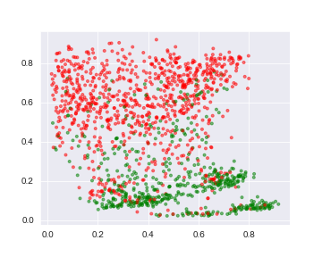
There are a few details to point out here. The red data points are points corresponding to Sale Price feature being less than its mean value and the green data points are points corresponding to Sale Price feature being more than its mean value. We can see that the green points are in two clusters. There are two arcs of the green points. The red data points are spread across the axes. Again, the seperation of the data points is not quite distinct. The scale of the encoded data points is not quite normal. That’s because the task of the autoencoder is to reconstruct the input, so anything in middle might not be the most accurate representation of the data.
It is clear that we have lost a lot of information in the process of encoding 276 features into 2 features. But with better model architecture and hyperparameter tuning better results can be achieved. An alternative to Autoencoders is Principal Component Analysis (PCA). The principal component analysis is a more theoretical linear algebraic approach which does a good job in retaining information of the original data. The eigenvalues and eigenvectors play a big role in retaining the information and mapping it to a smaller latent data space. The autoencoders on the other hand are neural networks which learn the mapping from the input to the input. So they are not focusing on retaining information from the original data, they are just looking for patterns in the data to map it from original data space to lower dimensional space and back to the original data space again. So both the methods differ in its core ideology.
Autoenecoders are computationally expensive than principal component analysis and are also difficult to create as there are many configurations one can try. But with proper architecture and optimizers, autoencoders can most of the time perform better than principal component analysis. Also, principal component analysis is a method of performing dimensionality reduction whereas autoencoders are a family of methods so it is more than capable of outperforming principal component analysis.
Principal Component Analysis is a good method to use when you want quick results and when you know that your data is linear. It is guaranteed to provide components which retain most of the variance of the data. Autoencoders are time consuming to develop and often require fine tuning the hyperparameters. Both of them have their perks and are useful in many scenarios.