Housing Price Analysis
The data used for the housing price analysis
came from Kaggle. You can find it here. When I first looked through the data,
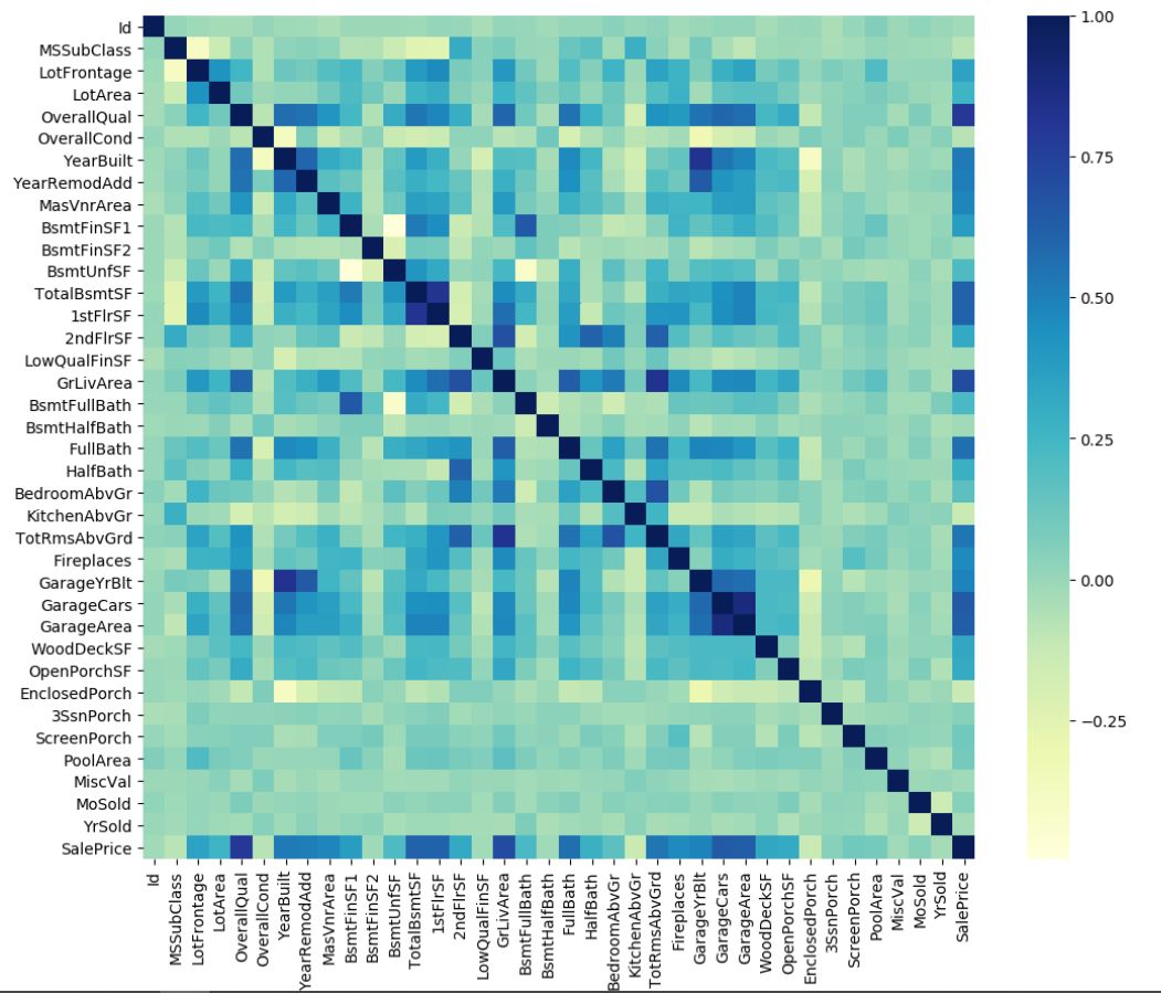
I got nervous due to the size of the dataset. There are a total of 80 features excluding the ID. This was the first time I dealt with a dataset of this size. I plotted a heatmap of the correlation of my features using the dataframe.corr() and sns.heatmap() methods. The heatmap came out to be like this:
I am not big into the Housing sector so my domain knowledge was little. I do have common sense and so I know that size of the house positively affects the price. When I glanced the dataset, there were a few fields that stood out to me,
- LotArea
- SaleCondition
- MasVnrArea
- OverallQual
I knew that these fields were gonna affect the Sale Price directly. My very first model was a Linear Regression Model with all of the features except for the ID and the target variable, SalePrice.
I defined a function nanCheck which would check for the nan values in the supplied dataframe and if any nan is found, it would set that entry to zero. I used scikit learn’s Label Encoder
to encode strings to integers to ensure compability with Linear Regression
model. I prepared my training and my testing data using train_test_split from sklearn.
Sklearn’s LinearRegression model was fitted with the training data and predicted on the testing data. The metric I used for evaluation is Root Mean Squared Logarithmic Error (RMSLE). I got a RMSLE of 0.20255. I was surprised to get a RMSLE as low as 0.2. I knew that this was an easy dataset and hence I wanted to bring the RMSLE closer to zero.
This was my baseline. Once I reached this point, I decided to get back into theory and read research papers and articles. I read about dimensionality reduction techniques such as Principal Component Analysis(PCA) and also learned about feature selection techniques. Once I was done reading and felt comfortable about improving my model, I got back into it.
Before I was using Label Encoder to turn my categorical features into numerical. After studying, I used one hot encoding using pandas.get_dummies. I did this because turning categorical data to numerical can be interpreted as some sort of ranking system by our model. I wrote a quick for loop for this :
for val in object_Val:
    df= pd.get_dummies(df, columns=[val])
Once I one hot encoded my categorical features, my column size grew. I had 289 columns now. I read somewhere that having more columns is better than having more rows as it provides more features for the model to work on.
After one hot encoding, I standardized my dataset using from sklearn.preprocessing import StandardScaler.
I implemented feature selection using the LassoCV model from sklearn. Using the Lasso model, I came down to 97 features. I wanted to apply the dimensionality reduction technique I just learned, PCA. I did so using sklearn’s library. I reduced my features to just 10.
Once I had done all this, I split the dataset into train and test. I initialised a random forest regressor. Evaluating the model with root mean squared logarithmic error, I got a score of 0.17
Though this wasn’t a huge improvement, it is an improvement. That being said, I have retreated to reading research papers and doing courses on DataCamp to learn more about this vast field.
I am currently working with a friend on Ada County Hosuing Analysis project. I will post about it after we have evaluation scores.